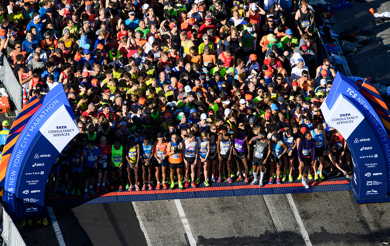
Have you ever wondered how the ranking system of the New York City Marathon works? Do the organizers stand at the finish line, trying to register numbers (race bibs) and finish times of the thousands of runners flowing in non-stop? Not really.

As may be expected, technology is the answer here, most professional races use some sort of radio frequency (also called “chip”) timing system (https://en.wikipedia.org/wiki/Transponder_timing) that automatically detects runners and reads their unique IDs as they pass through the receivers set up at the finish line.

I was experimenting with a home-made version of this technology a couple of years ago, building my own system called mind-the-GAP, suitable for smaller races where renting professional equipment is not an economically viable option.

Splits

I will not go through the details of the whole system in this article but rather focus on one recent addition I have been working on which allows the tracking of splits and also opens up the possibility to predict the runner’s current position.

Usually the full length of a race track is split into shorter sections and tracking equipment is placed at these milestones as well (in addition to the critical one at the finish line) to provide more detailed measurements about how the runners progressed through the course, also to serve as a safeguard against fraud, i.e., some participants cutting a few kilometers. 

Organizers of a 3K race that consist of two 1.5K sections back and forth for example probably want to put an additional receiver at 1.5K. If there is a longer race that runs through a whole city in a series of loops, organizers usually measure split times at various locations.

Predictions based on split data

Beside serving as data for detailed post-race performance analysis, the measured split times can be utilized during the race as well. The path of the race track is known in advance, if we also know the time when the runner passed by at the 5K-10K-15K markers, we can actually calculate the average speed of their progress and predict not only when they will reach the next (20K-25K etc.) marker but also estimate their current position on the race track. 

Knowing the runners approximate position and sharing this information with 3rd parties online (restricted to users whom the runner gave authorization to) might become handy in various scenarios, for example spectators can keep checking the progress of their friends or family members participating in the race.

Test environment

In preparation for implementing this prediction feature in mind-the-GAP, I was focusing on polishing the algorithm itself, working with simulated race data and observing the results as well as evaluating the accuracy of the prediction.

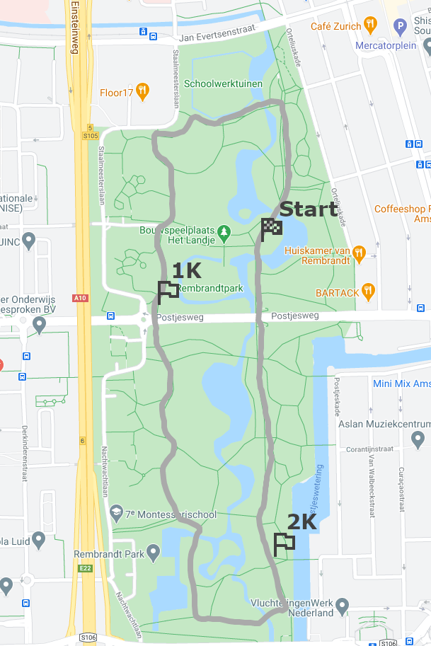
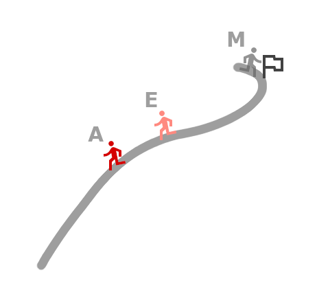
To have a race track for testing purposes, I have recorded a loop in Rembrandtpark, Amsterdam, a place where I used to go for runs myself. Coming from my phone’s GPS  receiver, the path is not extremely accurate, however, for the purpose of this exercise the recorded coordinate series is sufficient to serve as the race track that the imaginary runner of the simulation must progress through. I also marked a few split locations, where the race timing equipment would be placed in case of a real race. These are the 1K, 2K markers and the start/finish line at 2.66K. For implementing the prediction logic we do not need actual equipment placed in the park though, we will just assume that the performance of the runners will be measured at these locations.

Beside having the track path, we also need a test data set for the progression of the runner. This is a series of time-stamped coordinates that would simulate the race participant following the path of the track at their own pace.

We could also use this data to extract race timing measurements at the marked splits (let’s call it M or ‘measured position’) as well as keep tracking where the runners actually were during the race (let’s call it A for ‘actual position’). Of course the prediction uses solely M as input, A is only a reference set to be compared to the series of positions we estimate for the runner as an output of the prediction algorithm (let’s call it E for ‘estimated position’)

For this purpose I recorded an approximately 10K long series while running on the test race track in Rembrandpark. I was trying to keep an average pace of 5:15 with more or less consistency (varies between 5:05 and 5:30). These shifts in my performance could also demonstrate how the pace variations affect the accuracy of the prediction.

Note: pace shows how much time it takes to run 1KM, often used by runners as a measurement of target performance. When working on the implementation we could convert pace to speed and vice versa using a formula.

Building the test environment

For benchmarking the prediction algorithm with the recorded test data I implemented a Java application that simulated the race, processed the measured coordinates M and created the series of entries for the actual and estimated positions (A and E respectively). For displaying the simulation results I also added a simple website with Google Maps Javascript API integration to the project.

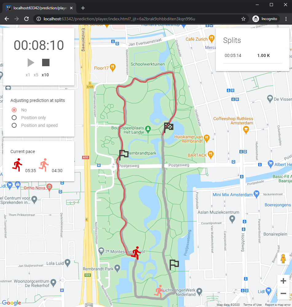
The path for the race track can be drawn as a series of latitude-longitude pairs as a base (in gray), then we draw both the actual and the estimated position of the runner on an other layer. The actual position (red) is what we got from the test GPS recording to see how well the estimation works, while the predicted position (soft red) is the output of the prediction algorithm implemented in Java.

For the JS player I am using a virtual clock, meaning that we could progress time faster or slower as we please, depending if we want to go through the course of the ~10K length of data very quickly or to observe some sections in more detail.

While iterating on the algorithm I have created multiple prediction series with various levels of adaptivity (no adjustment, position adjustments, position and speed adjustments), hence the UI also offers a control for switching between these modes to observe the simulation results for all three versions.

As a first demonstation, let’s see a test run for the most basic version, where no adjustments are happening, we simply take a constant assumed pace (4:30 in this case) and progress through the course of the race until it is over. As expected, the estimated position E is getting more and more ahead of actual A since the assumed pace was set too low intentionally (4:30 vs. 5:14), and there is no correction happening when receiving the measured values at split positions.

After having the basic predictor and the UI with the player already working, the whole idea of providing more accurate estimations based on the split measurements can be implemented with little effort. If real equipment were to be used, we could get updated performance data for the runners every time they pass a milestone where the sensors were placed. In case of the simulation, we could get this data extracted from my recorded run, using the timestamp of the entries recorded when I passed by the virtual markers (1K-2K-2.66K).

{ lat: 52.365500, lng: 4.847566, dist: 0, time: 0 },
{ lat: 52.364327, lng: 4.844433, dist: 1000000, time: 314 },
{ lat: 52.359670, lng: 4.847968, dist: 2000000, time: 644 },
{ lat: 52.365500, lng: 4.847566, dist: 2664000, time: 861 },
{ lat: 52.364327, lng: 4.844433, dist: 3664000, time: 1189 },
...

At the beginning of the virtual race, the pace for E can be still constant as in the first iteration, and later, as measurements coming at the milestones are incorporated into the calculations, we can adjust the estimated pace based on the actual progress of the runner.

What that means in practice can be shown with a simple example. If we were to assume 4:20 pace from the beginning, our runner would reach the 1K milestone at race time 00:04:20. However, if we get the mesurement for 10K at 00:05:14 instead, we’d know that the actual performance is worse than expected. So at the 1K milestone we just change the estimated pace to 5:14, then keep drawing the progression of E with this new speed, resulting in improved tracking accuracy. Obviously the more milestone measurement we got, the better the estimation will be.

Implementation-wise the logic is rather simple, at the beginning of the simulation we set E to the start line and initialize our predictor’s state, supplying the track’s shape (for moving E on the right path) as well as setting some initial pace that we think the runner will keep. As mentioned, for the demo we can set it to an intentionally low value to see its effect on the A-E difference.

The prediction algorithm is implemented as a loop, where we keep adjusting the estimated position of the runner as time progresses, either based on the incoming accurate M reading or simply updating the position based on the information that we have – the current state of the predictor and the shape of the track.

The core part of the prediction is implemented in predictor, where we  – depending on the availability of M – either adjust the current position and speed based on the received value, or simply advance the predicted position on the race track using the estimated speed of the runner. Let’s look into the relevant methods of state, where the calculations are happening:

public void updatePredictedPosition(PosEntry measurement) {
   estimatedPosOnTrack = measurement.distance % raceTrackLength;
}

public void updatePredictedSpeed(PosEntry measurement) {
   // New predicted speed: average speed for the last split
   long deltaT = clock.ts() - referenceMeasurement.timestamp;
   long deltaD = measurement.distance - referenceMeasurement.distance;
   if (deltaT <= 0 || deltaD <= 0) {
       throw new IllegalStateException("Invalid series");
   }
   estimatedSpeed = deltaD / deltaT;
}

public void advancePredictedPosition() {
   long deltaD = estimatedSpeed * clock.period();
   estimatedPosOnTrack = (estimatedPosOnTrack + deltaD) % raceTrackLength;
}

As noted in the updatePredictedSpeed() method, when updating the estimated speed of the runner, we only take the last two Ms into account (current measurement and previously passed reference measurement). We calculate the average speed for this last section and use it as speed prediction until we get a new measurement when the runner reaches the next split point. An alternative approach would be to calculate average speed for the whole race history or averaging multiple past splits with weights to compensate for outliers, e.g. one superfast section corrupting the speed estimate.

Simulation results

The simulation of my actual path vs. the predicted progress for the second and third iterations are shown below. As expected, at the beginning of the simulation the estimated position E is getting far ahead on the track of A, caused by the higher initial speed used for the estimation at the beginning. Later as we accumulate more and more measurements, E can get really close to A if we adjust both the position and the runner’s pace when receiving M values (in the 3rd iteration).

People experienced in analysis and statistics could also formulate some target function we could use to evaluate the accuracy of these predictions as well as compare them to various alternative approaches we could apply, which I will not do this time, but maybe in a follow-up article 🙂

The next (more practical) step for actual product development is to rather focus on incorporating this algorithm into the application core, where we could collect race timing measurements as well as predict all runners’ position almost real-time. Based on that we could also publish estimations via a web API or messaging system to be consumed by clients like a web frontend or a mobile application, reaching our end users eventually.